Orbital Mechanics: Kepler's Laws & Trajectories

Learning Goal: Master the complete mathematical, physical, and practical landscape of orbital mechanics and spaceflight physics. By completing this curriculum, you will build a robust intuition for spacecraft behavior, moving from classical Newtonian mechanics and Keplerian motion to complex interplanetary trajectory design (patched conics, gravity assists) and multi-body gravitational equilibria (Lagrange points).

• Prerequisites: High school physics (algebra-based) and basic calculus. Prior exposure to basic linear algebra (vectors and matrices) is helpful but not strictly required; foundational vector operations are covered within the course.
• Estimated Total Study Time: 35 Hours

---

Module 1: Coordinate Systems, Vectors, and Gravitational Foundations

This foundational module introduces the underlying classical mechanics and mathematical tools needed to model orbital trajectories. You will explore physical vectors, reference frames, and coordinate systems (such as the Perifocal and Geocentric-Equatorial frames) essential for spatial calculations, alongside a historical and mathematical review of Newton's Law of Universal Gravitation.

Recommended Videos

Why this video is valuable

This rigorous university lecture directly addresses the spatial math gap identified in early curriculum drafts. It introduces the fundamental mathematical objects of spaceflight: scalars, vectors, and "vectrices" (the matrix-based representation of coordinate frames). It provides a necessary bridge between pure vector calculus and the practical coordinate system transformations used to compute real-world spacecraft trajectories in three-dimensional space.

Knowledge Checkpoint

• Understand the mathematical distinction between a vector coordinate representation and a physical vector itself.
• Define a "vectrix" and explain how it simplifies coordinate frame transformations.
• Differentiate between inertial and non-inertial reference frames used in orbital calculations.

Why this video is valuable

Delivered by legendary physicist Richard Feynman, this classic lecture provides unmatched intuitive depth on the Law of Gravitation. Feynman expertly traces the intellectual leap from Kepler's observational, empirical laws of planetary motion to Isaac Newton's unified, mathematical theory of universal gravitation.

Knowledge Checkpoint

• Explain how Newton's Universal Law of Gravitation ($F = G \frac{m_1 m_2}{r^2}$) unifies terrestrial gravity with celestial orbits.
• Articulate the relationship between the inverse-square drop-off of gravity and the geometric properties of planetary paths.

Why this video is valuable

A highly-concentrated, clear refresher on the universal gravitation formula. This serves as a rapid mathematical baseline before diving into multi-body dynamics, highlighting the constants and variable relationships.

Knowledge Checkpoint

• State the units and value of the universal gravitational constant ($G$).
• Calculate the instantaneous gravitational force exerted between two spherically symmetric masses.

---

Module 2: Kepler’s Laws and Conic Sections

In this module, you will explore the geometry of orbital paths. You will learn how the gravitational mutual attraction of two bodies limits their paths to the family of curves known as conic sections: circles, ellipses, parabolas, and hyperbolas. You will study Kepler's three empirical laws and learn how they are derived directly from Newton's laws.

Recommended Videos

Why this video is valuable

This Ivy League physics lecture provides a mathematically rigorous derivation of Kepler's empirical laws using Newton's laws of motion and universal gravitation. It bridges the gap between historical geometry and calculus-driven classical mechanics, proving why orbits are bound to centripetal acceleration profiles.

Knowledge Checkpoint

• Derive the circular orbital velocity formula ($v = \sqrt{\frac{GM}{r}}$) from the balance of centripetal and gravitational forces.
• Explain how Kepler's Third Law ($T^2 \propto a^3$) mathematically emerges from Newtonian mechanics.

Why this video is valuable

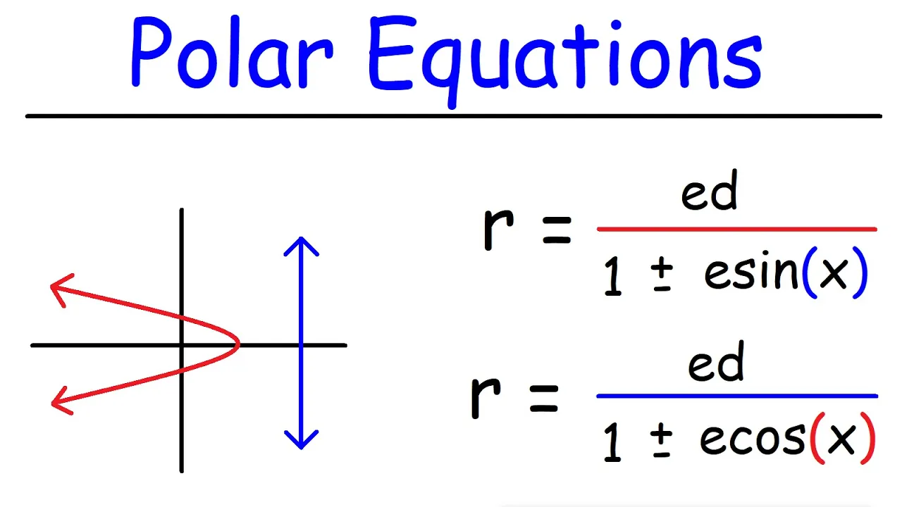
Orbits are computed almost exclusively using polar coordinates, where the central body serves as the origin (focus). This video provides the essential mathematical framework for defining ellipses, parabolas, and hyperbolas using polar equations ($r = \frac{ed}{1 \pm e \cos \theta}$), establishing the foundation for defining eccentricity ($e$) and true anomaly ($\theta$) in spaceflight.

Knowledge Checkpoint

• Define eccentricity ($e$) and identify the corresponding conic section for $e=0$, $0 < e < 1$, $e=1$, and $e > 1$.
• Sketch a conic section in polar coordinates given its eccentricity and directrix.
• Locate the coordinate origin (focus of the conic section) relative to the periapsis of an orbit.

---

Module 3: The Two-Body Problem and Orbital Elements

This module shifts focus to the classical Two-Body Problem ($2BP$), showing how we reduce the complex motion of two interacting massive bodies into an equivalent, solvable single-body system. You will also master the six Keplerian orbital elements used by astrodynamicists to uniquely define any orbit in three-dimensional space.

Recommended Videos

Why this video is valuable

This concise video breaks down the mathematical setup of the two-body problem. It uses Lagrangian mechanics to show how Newton's third law ($f_{21} = -f_{12}$) helps simplify the relative coordinate system between two masses ($m_1$ and $m_2$) into a single reduced mass moving around a static gravitational center.

Knowledge Checkpoint

• Define the "reduced mass" ($\mu = \frac{m_1 m_2}{m_1 + m_2}$) and explain why it is used in two-body dynamics.
• Formulate the basic equation of relative motion for the two-body problem.

Why this video is valuable

This segment addresses a major curriculum gap by providing a visual walkthrough of the six Keplerian orbital elements. Rather than just relying on mathematical symbols, it explains the spatial role of each parameter in defining an orbit's size, shape, plane tilt, alignment, and spacecraft position.

Knowledge Checkpoint

• List and define the six classical Keplerian orbital elements: Semi-major axis ($a$), Eccentricity ($e$), Inclination ($i$), Right Ascension of the Ascending Node ($\Omega$), Argument of Periapsis ($\omega$), and True Anomaly ($\theta$).
• Describe which orbital elements define the shape of the orbit, which define its orientation in 3D space, and which defines the location of the satellite.

Why this video is valuable

This video links orbital elements directly to vector state vectors ($\vec{r}$ and $\vec{v}$). It covers the perifocal coordinate system ($PQW$) centered on the periapsis vector, and explains how to transform these vectors back into the standard geocentric-equatorial reference frame.

Knowledge Checkpoint

• Define the $PQW$ (perifocal) coordinate frame axes relative to an elliptical orbit.
• Explain the steps required to convert a set of six Keplerian orbital elements into Cartesion position and velocity state vectors ($\vec{r}, \vec{v}$).

---

Module 4: Orbital Maneuvers and Coplanar Transfers

To navigate space, spacecraft must alter their velocity ($\Delta v$). This module teaches you how to compute the energy states of different orbits and perform orbital maneuvers. You will master coplanar orbital transfers, including the classic two-burn Hohmann transfer, plane changes, and how to optimize fuel budgets.

Recommended Videos

Why this video is valuable

This academic lecture addresses a gap in the review feedback by deriving the equations for orbital transfers. Instead of relying on approximations, it uses direct velocity-to-energy relationships ($v = \sqrt{\mu(\frac{2}{r} - \frac{1}{a})}$) to build step-by-step calculations for Hohmann transfer burns.

Knowledge Checkpoint

• Apply the Vis-Viva equation ($v^2 = \mu(\frac{2}{r} - \frac{1}{a})$) to calculate velocity at any point on an elliptical transfer orbit.
• Calculate the total delta-V ($\Delta v_{total} = |\Delta v_1| + |\Delta v_2|$) required to perform a Hohmann transfer between two nested circular orbits.

Why this video is valuable

This video provides an engaging, highly visual breakdown of Hohmann transfers. It explains how orbital mechanics can feel counter-intuitive—such as needing to burn prograde (speeding up) to drop into a different orbit—helping build strong mental models of orbital energy management.

Knowledge Checkpoint

• Explain why a Hohmann transfer requires exactly two discrete, impulsive engine burns.
• Describe the change in total orbital energy that occurs after the first burn and after the second burn of a Hohmann transfer.

Why this video is valuable

This practical guide uses Kerbal Space Program to show how real spacecraft rendezvous work. It demonstrates why simple target-chasing fails in orbit, and teaches you how to plan phase angles, match inclinations, and time transfer burns to successfully meet another orbiting object.

Knowledge Checkpoint

• Explain why burning directly toward a target in a shared orbit changes your altitude and causes you to drift further away.
• Outline the process of using a phasing orbit to catch up with or wait for a target spacecraft.

---

Module 5: Interplanetary Trajectories and Gravity Assists

This module moves beyond single-planet orbits to interplanetary flight. You will explore how astrodynamicists simplify complex multi-body spaceflight using the Patched Conics Approximation. This method divides an interplanetary journey into distinct, successive two-body segments dominated by a single body's Sphere of Influence ($SOI$). You will also study how gravity assists can redirect and accelerate spacecraft without using propellant.

Recommended Videos

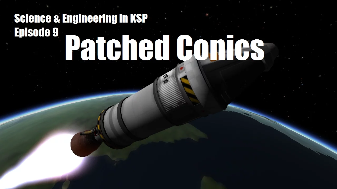
Why this video is valuable

This highly technical video directly addresses a key gap in the initial curriculum review. It provides step-by-step mathematical calculations for a patched conics trajectory, tracking how a spacecraft transitions from a planet's sphere of influence to a heliocentric transfer orbit, and finally into a target body's gravitational grip.

Knowledge Checkpoint

• Explain the core assumption of the Patched Conics Approximation.
• Calculate the hyperbolic excess velocity ($v_{\infty}$) of a spacecraft leaving a planet's sphere of influence.
• Match the departure velocity vector from a planet's parking orbit to the entry velocity vector of a heliocentric transfer trajectory.

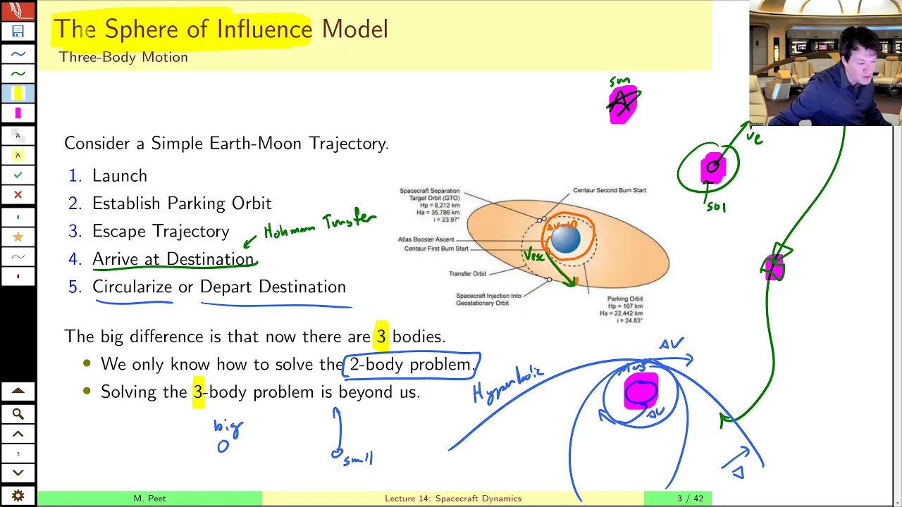
Why this video is valuable

This lecture explains the mathematical physics of the Sphere of Influence ($SOI$). It provides the Laplace derivation used to define the boundary where a planet's gravitational pull overtakes the Sun's background gravity, giving you the math needed to locate transition "patch points" during a mission.

Knowledge Checkpoint

• State and apply the Laplace formula for the radius of a planet's Sphere of Influence: $r_{SOI} \approx a \left(\frac{m_p}{M_s}\right)^{2/5}$.
• Explain why the patched conic approximation breaks down near the boundary of the Sphere of Influence.

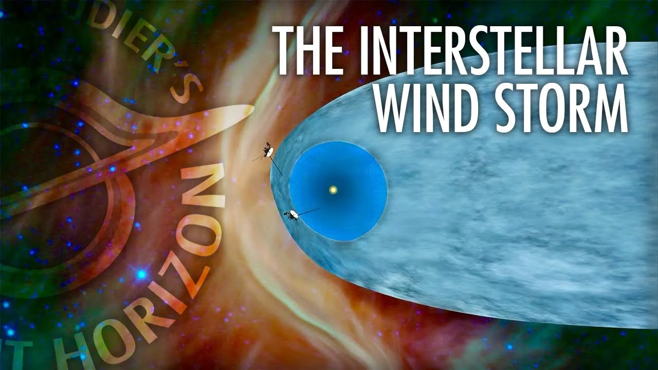
Why this video is valuable

Featuring Voyager project scientist Dr. Linda Spilker, this video discusses the practical realities of interplanetary navigation. It explains how Voyager utilized a rare planetary alignment to perform consecutive gravity assist (slingshot) maneuvers, showing how 3D velocity vectors change during a planetary flyby.

Knowledge Checkpoint

• Explain how a spacecraft gains speed relative to the Sun during a planetary flyby, even though its energy relative to the flyby planet remains constant.
• Describe how the entry angle (passing behind vs. in front of a planet's orbital path) determines whether a gravity assist accelerates or decelerates a spacecraft.

---

Module 6: The Restricted Three-Body Problem and Lagrange Points

This final module covers systems where a third body has negligible mass compared to two primary massive bodies. You will study the Restricted Three-Body Problem ($CR3BP$), locate the five gravitational equilibrium zones known as Lagrange points, and understand modern non-Keplerian orbits (like Halo and Lissajous orbits) used by spacecraft like the James Webb Space Telescope ($JWST$).

Recommended Videos

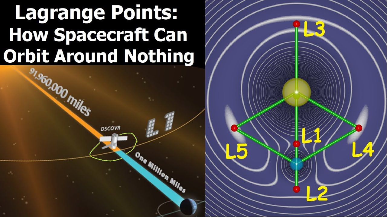
Why this video is valuable

Scott Manley provides an excellent conceptual and mathematical overview of Lagrange points. Using clear coordinate transformations, he shows how centrifugal and gravitational forces balance in a rotating frame of reference, explaining why these points exist and how spacecraft use them for stable observations.

Knowledge Checkpoint

• Identify the physical location of the five Lagrange points ($L_1$ through $L_5$) in a two-body system.
• Differentiate between collinear points ($L_1, L_2, L_3$) and triangular points ($L_4, L_5$) in terms of gravitational stability and the Coriolis effect.

Why this video is valuable

This video walks through the complete mathematical derivation of Lagrange Point 1 ($L_1$). Starting with force balance equations in a rotating reference frame, it applies a binomial approximation to solve the fifth-order polynomial, showing you the exact algebra behind locating these equilibrium zones.

Knowledge Checkpoint

• Set up the equation of motion for a third body of negligible mass experiencing gravitational forces from two primary bodies in a rotating coordinate system.
• Explain how the binomial approximation is used to simplify and solve for the distance of $L_1$ from the primary body.

Why this video is valuable

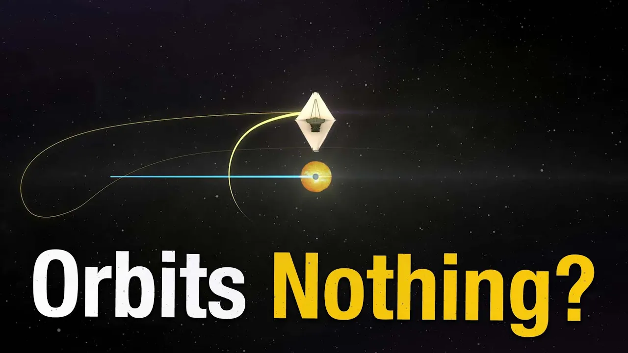
This video explains how spacecraft orbit Lagrange points where there is no physical mass. It details the geometry of Halo and Lissajous orbits, explaining why the James Webb Space Telescope orbits the Sun-Earth $L_2$ point in a wide three-dimensional path rather than sitting stationary at the point itself.

Knowledge Checkpoint

• Define a "Halo orbit" and explain how a spacecraft can orbit a mathematical equilibrium point with no central mass.
• Explain why the James Webb Space Telescope requires active station-keeping maneuvers to maintain its orbit around the unstable $L_2$ point.

---

Course Map

This flowchart shows the recommended learning path and module dependencies. Complete the modules in sequential order to build your mathematical and physical foundations before tackling advanced multi-body dynamics.

---

Key People Index

• Isaac Newton (1643–1727): Developed the laws of motion and universal gravitation, mathematically proving the physics behind Kepler's empirical observations.
• Johannes Kepler (1571–1630): Formulated the three empirical laws of planetary motion based on Tycho Brahe's observational data.
• Richard Feynman (1918–1988): Nobel laureate physicist whose lectures offer profound, intuitive insights into gravitational laws.
• Joseph-Louis Lagrange (1736–1813): Mathematician who resolved special cases of the three-body problem, identifying the five gravitational equilibrium points that bear his name.
• Dr. Linda Spilker: Planetary scientist and Voyager project scientist who helped design and execute the gravity-assist trajectories of the Grand Tour.
• Dr. Matthew Peet: Academic lecturer in aerospace engineering who provides the mathematical frameworks for state vector transformations and Sphere of Influence calculations.

---

Final Self-Assessment

Test your mastery of the curriculum by verifying that you can confidently complete each of the following tasks:

• Write down Newton's Law of Universal Gravitation in vector form and explain how it drives centripetal acceleration.
• Derive Kepler's Third Law ($T^2 \propto a^3$) starting from the balance of gravitational and centripetal forces for circular orbits.
• Determine the orbit type (circular, elliptical, parabolic, or hyperbolic) given only its eccentricity vector magnitude or orbital energy state.
• List all six classical Keplerian orbital elements and explain how they map to Cartesian position ($\vec{r}$) and velocity ($\vec{v}$) vectors.
• Calculate the total $\Delta v$ budget for a Hohmann transfer between two coplanar circular orbits using the Vis-Viva equation.
• Estimate the radius of a planet's Sphere of Influence ($SOI$) using its semi-major axis and the mass ratio of the planet to the Sun.
• Explain how a spacecraft gains heliocentric speed during a trailing-side planetary flyby (gravity assist).
• Calculate the position of the Sun-Earth Lagrange Point 1 ($L_1$) using binomial approximations of the gravitational force equations.
• Explain the difference between a stable ($L_4/L_5$) and unstable ($L_1/L_2/L_3$) Lagrange point, and describe the role of the Coriolis force in maintaining orbit stability.