DIY Spectrometer: Optics, Build & Calibration

Learning Goal: Construct a functional desktop spectrometer using a diffraction grating and digital camera, calibrating the device to identify chemical compounds based on emission spectra.

---

Prerequisites

• Basic understanding of algebra (linear equations for calibration).
• Familiarity with physical safety when working with household electricity, hot components, or open flames (for chemical testing).
• Standard computer environment to run analysis tools (web browser or a Python environment).

Estimated Study Time

• Total Estimated Time: 26 Hours (including optical theory, housing fabrication, software setup, calibration, and wet-lab testing).

---

Module 1: Physics of Light & Spectroscopy Foundations

In this introductory module, you will master the wave nature of light, explore the electromagnetic spectrum, and examine how atoms interact with energy. Understanding the distinction between continuous, emission, and absorption spectra is critical before building any optical instrumentation.

Recommended Videos

Why this video is valuable:

This lecture serves as a comprehensive starting point. It contextualizes light as an electromagnetic wave and clarifies how it occupies a narrow, visible region of the broader spectrum. It explains how spectrometers dissect this wave to reveal structural, chemical, and physical details of far-away or minute matter.

Knowledge Checkpoint:

• Understand why white light splits into a spectrum of colors when diffracted.
• Identify the approximate wavelength limits (in nanometers) of the visible light spectrum.
• Describe the difference between continuous light sources and discrete spectral lines.

---

Why this video is valuable:

This video breaks down the differences between three primary types of spectra: continuous, emission, and absorption. By correlating molecular state changes with spectral outputs, you'll gain the quantum mechanics intuition needed to interpret the bands of light your spectrometer captures.

Knowledge Checkpoint:

• Define a continuous spectrum and name a source that creates one (e.g., an incandescent bulb).
• Explain how an emission spectrum is created when excited atoms release energy.
• Contrast how absorption spectra appear compared to emission spectra under identical gas conditions.

---

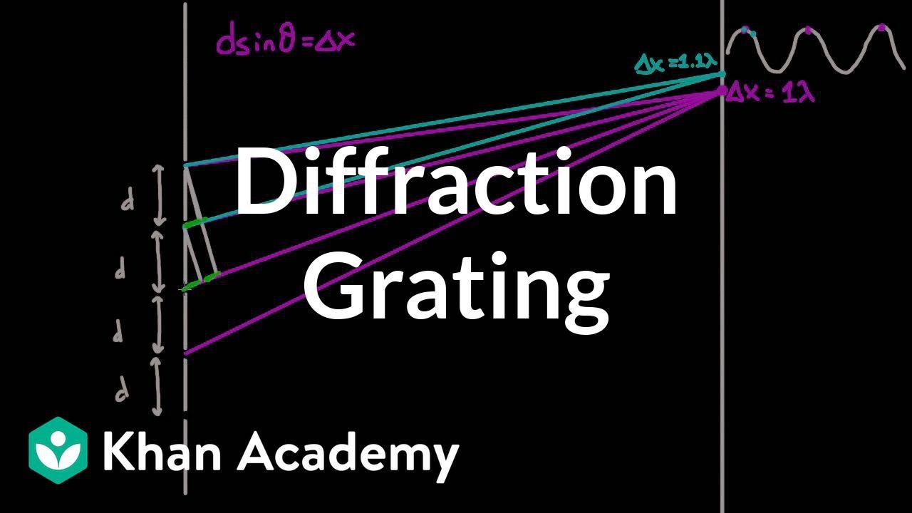
Why this video is valuable:

This deep dive from Khan Academy explains the mathematics and physics of diffraction gratings. It details how thousands of closely spaced parallel slits use wave interference to separate white light into sharply defined, localized color bands, preparing you for the engineering of your optical paths.

Knowledge Checkpoint:

• Explain how constructive and destructive interference produce bright and dark fringes.
• Understand why a grating produces more distinct, sharper lines than a simple double-slit setup.
• Trace the path of short wavelengths (violet/blue) versus long wavelengths (red) through a grating.

---

Module 2: Optical Components & Camera Sensors

To engineer a functional spectrometer, you must understand the hardware components. This module explains how optical slits determine instrument resolution, how diffraction gratings disperse wavelengths according to the grating equation, and how digital image sensors (CMOS/CCD) translate analog wavelengths into color channels using Bayer filters.

Recommended Videos

Why this video is valuable:

This quick revision focuses on the diffraction grating equation: $n\lambda = d \sin(\theta)$. Understanding how to calculate the distance between slits ($d$) and physical deflection angles ($\theta$) is crucial when calculating the physical dimensions of your spectrometer housing.

Knowledge Checkpoint:

• State the diffraction grating equation and identify what each variable ($n$, $\lambda$, $d$, $\theta$) represents.
• Convert a grating specification of "lines per millimeter" into the physical slit-spacing distance $d$.
• Calculate the expected angle of first-order diffraction ($n=1$) for a green light wavelength of 532 nm.

---

Why this video is valuable:

Digital sensors do not inherently perceive color; they measure raw light intensity (luminance). This video explains how the Bayer filter array sits over physical CMOS/CCD pixels to isolate Red, Green, and Blue channels. This understanding is key for processing camera data in later software stages.

Knowledge Checkpoint:

• Explain why the Bayer pattern uses a 2:1:1 ratio of green, red, and blue filters.
• Understand "demosaicing" and its impact on color interpolation at sharp intensity borders.
• Identify how a digital sensor turns analog photon strikes into separate Red, Green, and Blue pixel intensity values.

---

Why this video is valuable:

This technical lecture explains the relationship between mechanical slit width, diffraction grating angles, and optical resolution. It outlines how slit-width choices dictate the limits of your system’s resolving power ($\mathcal{R} = \frac{\lambda}{\Delta\lambda}$).

Knowledge Checkpoint:

• Explain the trade-off between optical resolution (sharp lines) and light throughput (brightness) when choosing slit width.
• Identify the function of the collimator lens in ensuring parallel rays strike the diffraction grating.
• Describe how wider slits can cause distinct, closely-spaced spectral lines to blend together.

---

Why this video is valuable:

This short clip illustrates the physical effect of a slit's aperture size. It visualizes how limiting the width of a light source minimizes stray overlaps, showing why a narrow physical slit is essential to prevent spectral smearing.

Knowledge Checkpoint:

• Visualize how a wide aperture lets multiple overlapping angles of light pass, reducing line sharpness.
• Identify why a physical slit must have straight, clean, and parallel edges.

---

Module 3: Constructing the Physical Spectrometer Housing

This module guides you through building your spectrometer housing. You can construct this chassis out of everyday materials like cardboard or utilize 3D printing. The primary goal is aligning the slit, diffraction grating, and camera sensor while eliminating stray light reflections that could degrade your data.

Recommended Videos

Why this video is valuable:

This classic construction guide from Public Lab details how to build a basic visible-light spectrometer using a DVD (acting as a transmission diffraction grating), a webcam, black cardboard paper, and an enclosure. It offers a practical layout template you can replicate at home.

Knowledge Checkpoint:

• Learn how to safely split a standard DVD-R to isolate its internal, microscopic diffraction tracks.
• Position the camera relative to the diffraction grating and light slit at a 45-degree angle to catch the first-order diffraction beam.
• Construct a uniform, parallel-edged entry slit using thick black paper cardstock.

---

Why this video is valuable:

An MIT OpenCourseWare demonstration showing how to build an entry-level spectrometer using foam board and a CD. Crucially, it highlights using industrial razor blades to construct an adjustable entry slit, which provides the clean, parallel borders needed for high resolution.

Knowledge Checkpoint:

• Observe how dual razor blades can be mounted to create a micrometric, adjustable entry slit.
• Identify how subtle changes in the distance between the slit and the grating affect the spread of the spectrum.
• Secure physical components to prevent internal shifts from ruining your wavelength calibration.

---

Why this video is valuable:

A key challenge when building DIY spectrometers is dealing with stray light reflecting inside the chassis. This engineering video defines the types of stray paths (such as ghost images and scattering bounces) that reach your sensor, helping you design a light-tight housing.

Knowledge Checkpoint:

• Distinguish between a "straight shot" (leak) and scattered light bouncing within the chamber.
• Understand why lining the inner walls of your spectrometer housing with matte black felt, paper, or paint is critical.
• Identify how unexpected internal surface reflections can introduce false peaks into your captured data.

---

Why this video is valuable:

If you have access to a 3D printer, this video introduces how to use OpenSCAD to design precise, repeatable 3D-printable spectrometer housings. It emphasizes the importance of alignment, spacing, and clean mounting points.

Knowledge Checkpoint:

• Understand how 3D design files allow you to set rigid, fixed alignment distances between your slit, grating, and sensor.
• Design integrated paths to slide in calibration filters or sample cuvettes.

---

Module 4: Software Integration & Wavelength Calibration

Now that your physical spectrometer is built, you must convert the camera's 2D image feed into digital data. This module focuses on extracting a 1D spectral intensity profile from 2D camera images and calibrating raw pixel column numbers into real nanometer wavelengths using known mercury emission lines from a fluorescent lamp.

⚠️ CRITICAL WARNING FOR SELF-STUDY: Some search queries for "software calibration" can return videos about a musical instrument called a "Theremini" (such as Videos 18 and 38). These are synthesizer calibrations and have nothing to do with optical spectroscopy. Always skip musical Theremin videos.

Recommended Videos

Why this video is valuable:

This tutorial walks you through Public Lab's open-source browser utility, "Spectral Workbench". It shows you how to connect your webcam, align a digital crosshair over your active light diffraction strip, and capture real-time, digitized intensity peaks.

Knowledge Checkpoint:

• Connect a live USB camera to a browser-based analysis platform.
• Define the Region of Interest (ROI) line across the center of your visible spectral band.
• Learn how to export intensity values as raw CSV data for further processing.

---

Why this video is valuable:

This video shows you how to calibrate your spectrometer. It explains how to point your device at a standard compact fluorescent lamp (CFL), capture its characteristic mercury vapor emission peaks, and map those peaks to their known scientific wavelengths (e.g., 435.8 nm and 546.1 nm) to calibrate your system.

Knowledge Checkpoint:

• Identify the blue (435.8 nm) and green (546.1 nm) mercury spectral lines in a live CFL emission profile.
• Map pixel column coordinates to known wavelengths using a linear equation ($y = mx + b$).
• Verify calibration accuracy by testing against a secondary reference source, such as a known laser pointer.

---

Why this video is valuable:

This short demonstration explains the logic of spectrum extraction. It shows how software isolates a horizontal row of pixels in a 2D digital image, extracts the RGB color values across those pixels, and plots them as an intensity curve.

Knowledge Checkpoint:

• Visualize how a horizontal slice of a 2D camera sensor represents a scale of increasing wavelengths.
• Understand how to plot raw pixel columns on the X-axis against intensity values (0-255) on the Y-axis.

---

Deep Dive: Custom 1D Spectral Extraction Code

If you prefer to write custom code instead of using web-based software, you can use Python with OpenCV to extract spectral data. Here is the process:

import cv2 import numpy as np import matplotlib.pyplot as plt

1. Load the 2D spectral image captured from your webcam

img = cv2.imread('calibration_cfl.png')

2. Define a horizontal region of interest (ROI) across the center row

Let's average a 10-pixel tall band to minimize camera noise

height, width, _ = img.shape row_start, row_end = int(height/2 - 5), int(height/2 + 5) roi = img[row_start:row_end, 0:width]

3. Convert to grayscale to obtain overall intensity, or extract individual color channels

gray_roi = cv2.cvtColor(roi, cv2.COLOR_BGR2GRAY) intensity_profile = np.mean(gray_roi, axis=0) # Average vertically within our 10px strip

4. Plot pixel index (X) vs. Light Intensity (Y)

plt.figure(figsize=(10, 4)) plt.plot(intensity_profile, color='black') plt.xlabel('Pixel Column Index') plt.ylabel('Intensity Value (0-255)') plt.title('Raw 1D Spectrum Profile') plt.grid(True) plt.show()

Calibration Math

Once you identify the pixel columns corresponding to the primary mercury peaks, apply a linear fit: $\lambda = m \cdot (\text{Pixel Column}) + b$

For example, if you find the blue peak ($435.8\text{ nm}$) at Pixel 120 and the green peak ($546.1\text{ nm}$) at Pixel 340:

1. Calculate slope: $m = \frac{546.1 - 435.8}{340 - 120} = 0.5014\text{ nm/pixel}$
2. Solve intercept: $b = 435.8 - (0.5014 \cdot 120) = 375.63\text{ nm}$
3. Your calibration formula is: $\lambda = 0.5014 \cdot (\text{Pixel}) + 375.63$

---

Module 5: Chemical Identification & Spectral Analysis

In this final module, you will put your calibrated spectrometer to work. You will learn to perform flame tests using metal salts, capture emission spectra, and search the NIST atomic spectra database to match your experimental peaks to specific chemical compounds.

Recommended Videos

Why this video is valuable:

This laboratory guide demonstrates safe flame tests using various metal salts. It illustrates how thermal excitation prompts electrons to jump to higher shells, emitting distinct visible wavelengths as they fall back to ground states.

Knowledge Checkpoint:

• Learn the safety protocols for performing metal salt flame tests (such as copper, sodium, and strontium).
• Connect the visual flame color to the dominant emission peak wavelengths your spectrometer will see.
• Identify which elements yield clean, easily recognizable emission lines for home testing.

---

Why this video is valuable:

This clip introduces the National Institute of Standards and Technology (NIST) Atomic Spectra Database. It demonstrates how to search for elements using their chemical symbols and ionization states, helping you locate reference spectral tables to verify your experimental findings.

Knowledge Checkpoint:

• Navigate the NIST database to find specific elemental emission lines.
• Understand the notation of ionization states (e.g., Na I represents neutral sodium).
• Filter database results by visible light range ($400\text{ nm}$ to $700\text{ nm}$) to match what your digital sensor can capture.

---

Why this video is valuable:

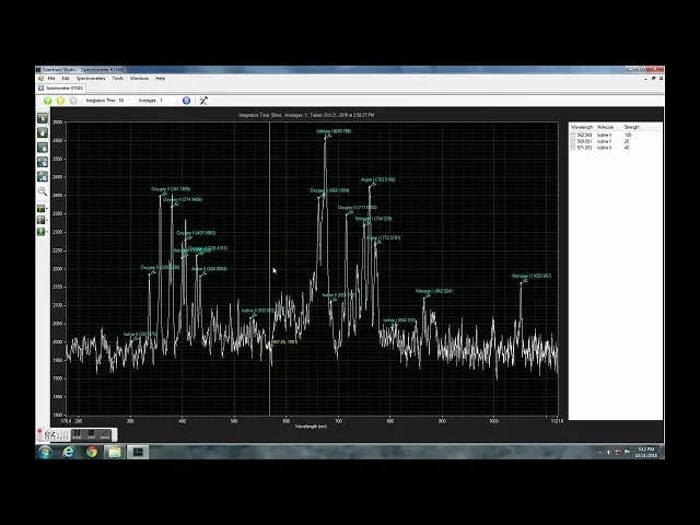
This video showcases a practical home experiment using high-voltage arcs and chemical excitation. It demonstrates how to analyze physical samples using emission spectroscopy and compares DIY measurements with established database standards.

Knowledge Checkpoint:

• Learn how to extract clean emission data from excited chemical samples without saturated highlights.
• Compare experimental spectrum profiles against known database peaks to identify unknown samples.

---

Step-by-Step Guide: Matching DIY Peaks to the NIST Database

Because DIY spectrometers have limited resolution compared to laboratory-grade instruments, you will rarely match a NIST line with 100% precision. Follow this guide to reconcile your data:

[DIY Spectrum Sample] [NIST Reference Database] Peak observed at: 589.6 nm =============(± 3 nm)=============> Strong Line: Na I (589.0 nm & 589.6 nm) (Doublet appears as single 589 nm peak)

1. Calculate the Resolution Limit of your Instrument ($\Delta\lambda$): Look at your calibrated CFL emission plot. Check the width of the green line ($546\text{ nm}$) at half of its maximum intensity (known as Full Width at Half Maximum, or FWHM). If that peak is $6\text{ nm}$ wide, your instrument resolution $\Delta\lambda \approx 6\text{ nm}$.

2. Retrieve Reference Lines from the NIST Database:

   • Go to the NIST Atomic Spectra Database Lines Form.
   • Enter your target element (e.g., Na for Sodium) in the Spectrum input.
   • Set the limits of your search to the visible region: Wavelength Range: 400 to 700 nm.
   • Under Transition Strength, choose to show relative intensities. Click Retrieve Data.

3. Reconcile High-Resolution Doublets with Low-Resolution Peaks: The NIST database lists two strong, distinct lines for neutral Sodium (Na I) at $589.0\text{ nm}$ and $589.6\text{ nm}$.

   • Because your spectrometer's resolution limit ($\Delta\lambda \approx 6\text{ nm}$) is wider than the distance between these lines ($0.6\text{ nm}$), they will merge into a single broad peak on your sensor.
   • Calculate the intensity-weighted average of these close reference lines: $\lambda_{\text{combined}} = \frac{\sum (\lambda_i \cdot I_i)}{\sum I_i}$ Where $\lambda_i$ represents the individual wavelengths and $I_i$ is their intensity value listed in the database.
   • Compare this combined average ($589.3\text{ nm}$) to your measured peak ($589.6\text{ nm}$). An error within $\pm 1.5\text{ nm}$ indicates a successful chemical identification.

---

Course Map

---

Key People Index

• Gustav Kirchhoff & Robert Bunsen (1848): Developed modern spectroscopy, proving that each chemical element produces a unique, characteristic set of emission lines.
• Isaac Newton (1666): Used prisms to demonstrate that white light is a mixture of separate color wavelengths, laying the groundwork for optical dispersion.
• Bryce Bayer (1975): Patent holder of the Bayer filter mosaic, which allows digital camera sensors to capture red, green, and blue light channels.
• William Hyde Wollaston & Joseph von Fraunhofer (Early 1800s): Discovered and mapped dark absorption lines (Fraunhofer lines) in the spectrum of sunlight, pointing the way to atomic absorption theory.

---

Final Self-Assessment

Complete this checklist to verify that you have successfully constructed, calibrated, and utilized your spectrometer:

• Theory: Can you write the diffraction grating formula and solve for the diffraction angle $\theta$ of a known wavelength?
• Resolution: Can you explain how the width of your entry slit affects your system's overall optical resolution?
• Bayer Filters: Can you explain why digital cameras must use software interpolation (demosaicing) to yield clean, full-color spectral lines?
• Light Isolation: Is your spectrometer chassis completely sealed against light leaks, with the interior surfaces coated in matte black to prevent internal reflections?
• Digital Extraction: Can you isolate a 2D digital photograph of a spectrum, select a single row of pixels, and plot those pixel columns against their brightness values?
• Calibration Source: Have you identified the characteristic $435.8\text{ nm}$ and $546.1\text{ nm}$ mercury emission peaks in a fluorescent lamp's spectrum?
• Linear Fit: Have you mapped your camera's pixel coordinates to physical wavelengths (in nanometers) using a linear equation?
• Testing: Have you captured the bright orange emission line of a Sodium salt flame test and matched it to the Na I line in the NIST database?
• NIST Reconciling: Do you know how to calculate a weighted average of close reference wavelengths in the NIST database to match them with the lower-resolution peaks of your DIY device?