Stochastic Calculus: Brownian & Black-Scholes

Learning Goal: Build the complete mathematical foundations of continuous-time stochastic processes—progressing from discrete random walks to Brownian motion, establishing the rigorous framework of Itô calculus, deriving Itô's Lemma, and ultimately constructing and solving the Black-Scholes-Merton option pricing model.

• Prerequisites: Multivariable calculus (derivatives, partial derivatives, Taylor series expansions) and introductory probability (expectation, variance, and probability density functions).
• Estimated Total Study Time: 18 Hours

---

Module 1: Foundations of Probability & Calculus

To understand stochastic processes, we must first master the language of probability and continuous limits. This module reviews the continuous random variables, probability density functions (PDFs), expectations, and continuous limits that form the core foundations of stochastic calculus. Crucially, it bridges the gap between pure mathematics and its direct applications in quantitative finance.

Recommended Videos

Why this video: This video serves as a targeted calculus refresher specifically designed for quantitative finance. It replaces generic high-school level material with a focused look at continuous limits, derivatives, and linear approximations ($df \approx f'(x)dx$) through the lens of quant interviews and stochastic foundations.

---

Why this video: Before entering continuous space, you must possess an intuitive grasp of random variables. This classic lecture provides the essential distinction between discrete and continuous random variables, illustrating how they map experimental outcomes to real numbers.

---

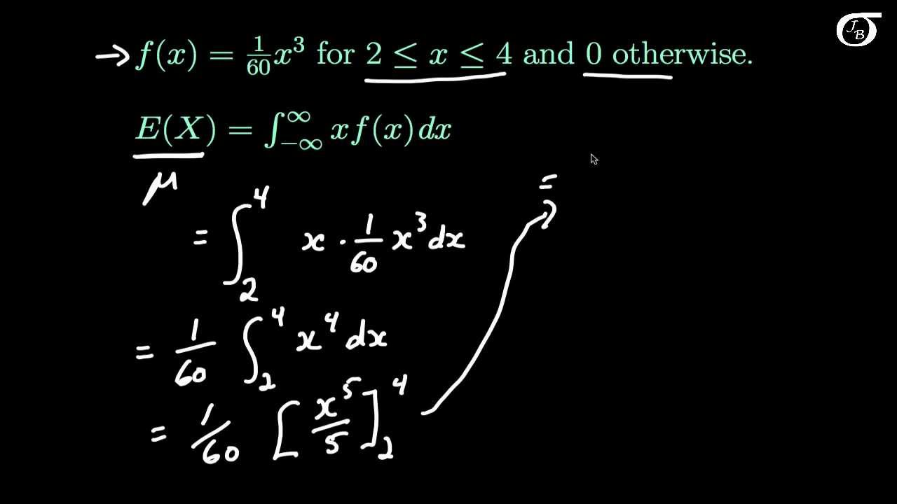
Why this video: Stochastic integration relies heavily on calculating expectations of continuous paths. This video provides step-by-step mathematical proofs of how to calculate the mean (expectation) and variance of continuous distributions using integrals over probability density functions (PDFs).

Knowledge Checkpoint

• Define a random variable mathematically as a mapping from a sample space to the real numbers.
• Set up and evaluate the Riemann integral for the expectation $\mathbb{E}[X]$ and variance $\text{Var}(X) = \mathbb{E}[X^2] - (\mathbb{E}[X])^2$ of a continuous random variable.
• Understand the concept of a limit in calculus and how derivatives represent localized linear operators.

---

Module 2: From Random Walks to Brownian Motion

Brownian motion (or the Wiener process) is the mathematical bedrock of continuous-time stochastic models. This module demonstrates how a discrete-time random walk (like a sequence of coin flips) transforms into a continuous-time Brownian motion when time intervals shrink to zero. You will explore its unique properties, including independence of increments and normal distribution scaling.

Recommended Videos

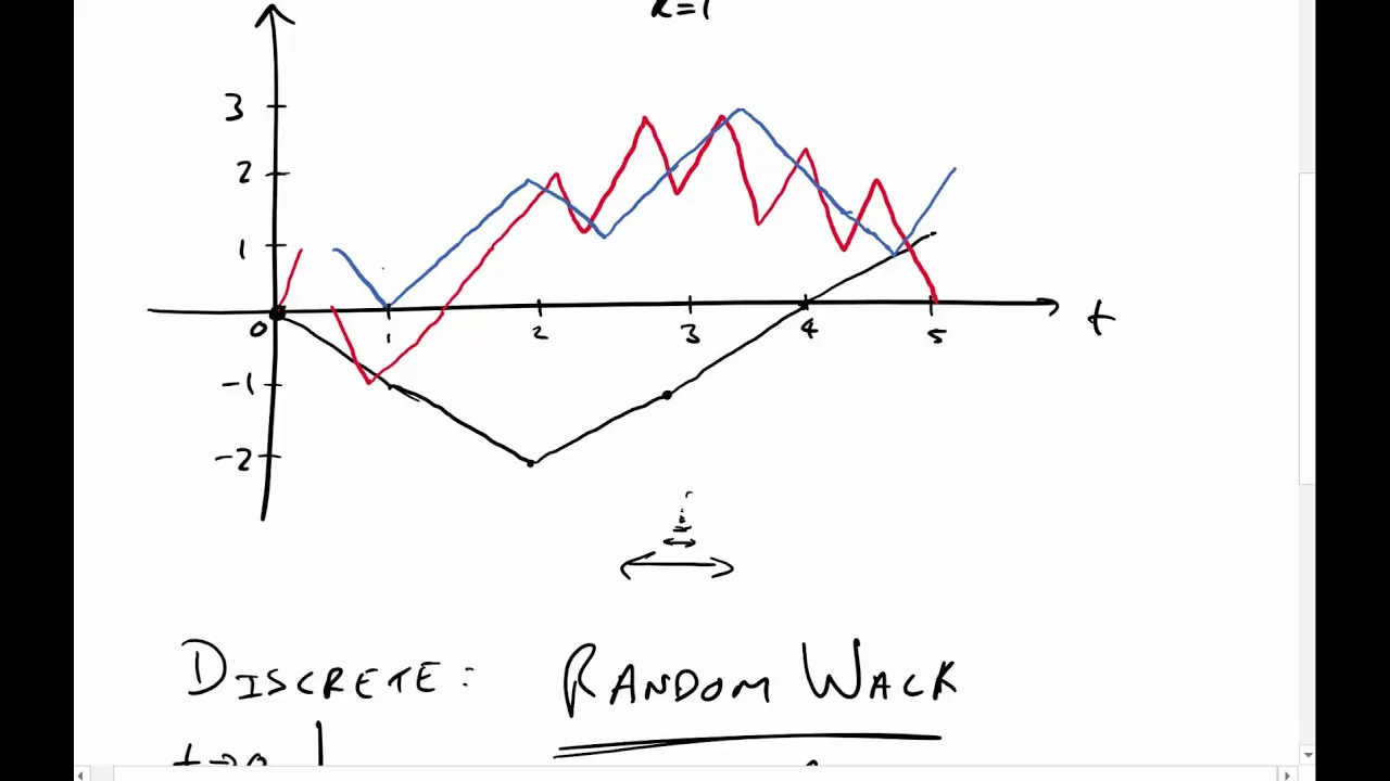
Why this video: Professor Bill Byrne provides an elegant, highly intuitive bridge from discrete coin-flipping random walks to continuous Brownian motion. He outlines the dual scaling limits required: converting discrete increments to normal increments and dividing time into $n$ microscopic parts.

---

Why this video: For those seeking a deeper mathematical dive, this lecture formally models the scaling limit of a symmetric random walk. It walks through the math proving why the mean remains zero while the variance scales perfectly with time as the step size approaches zero.

---

Why this video: This video clearly details the formal axioms defining a standard Wiener process ($W_t$): starting at zero, almost-sure path continuity, independent increments, and stationary normal increments where $W_t - W_s \sim \mathcal{N}(0, t - s)$.

Knowledge Checkpoint

• Explain the two key mathematical scaling conditions needed to transition a symmetric random walk to a Wiener process.
• List the four foundational mathematical axioms of standard Brownian motion.
• Prove why the variance of a Brownian increment over a time window of size $\Delta t$ is exactly equal to $\Delta t$.

---

Module 3: The Itô Integral & Stochastic Integration

Classical Riemann-Stieltjes integration fails spectacularly when applied to Brownian paths. Why? Because Brownian motion is highly erratic, exhibiting infinite total variation. This module introduces the concept of Quadratic Variation—proving that while a Brownian path has infinite first variation (making it nowhere differentiable), its quadratic variation over $[0, t]$ converges deterministically to $t$. This discovery lays the groundwork for the Itô integral, defined via left-endpoint Riemann sums, and its central tool: the Itô Isometry.

Recommended Videos

Why this video: This video provides an engaging, thorough mathematical introduction to the Riemann-Stieltjes integral ($\int f(x) dg(x)$). Before learning why classical integration fails for stochastic processes, you must first understand how integration with respect to a non-linear function works in a deterministic setting.

---

Why this video: This video directly bridges the gap regarding Quadratic Variation. It mathematically demonstrates how the sum of squared increments $\sum (W_{t_{i+1}} - W_{t_i})^2$ converges almost surely to $T$ as the mesh size of the partition approaches zero, and explains why this infinite variation prevents Brownian paths from being differentiable.

---

Why this video: This core lecture from MIT OCW establishes the formal definition of the Itô stochastic integral. It highlights why we evaluate the integrand strictly at the left endpoint of each subinterval (to preserve non-anticipating/adapted behavior) and contrasts it with classical integration.

---

Why this video: This video directly addresses the gap regarding the Itô Isometry. It provides a step-by-step mathematical proof: squaring the Itô integral and taking the expectation, demonstrating how cross-terms cancel out due to independent increments, resulting in the fundamental identity: $\mathbb{E}\left[ \left(\int_0^T X_t dW_t\right)^2 \right] = \mathbb{E}\left[ \int_0^T X_t^2 dt \right]$.

Knowledge Checkpoint

• Define the quadratic variation of a continuous process and write down its deterministic value for standard Brownian motion over $[0, t]$.
• Explain why a non-zero quadratic variation prevents us from using classical Riemann-Stieltjes calculus to integrate along Brownian paths.
• State the definition of the Itô integral and identify why the left-endpoint evaluation is crucial for maintaining the martingale property.
• Write down the Itô Isometry formula and explain how it simplifies the calculation of variance for stochastic integrals.

---

Module 4: Itô's Lemma: The Chain Rule of SDEs

In classical calculus, the chain rule allows us to differentiate composite functions: $df(x) = f'(x)dx$. In the stochastic realm, because $(dW_t)^2 \approx dt$ is non-negligible (due to quadratic variation), Taylor series expansions cannot be truncated at the first-order term. This module derives and teaches you how to apply Itô's Lemma—the stochastic equivalent of the chain rule.

Recommended Videos

Why this video: Bill Byrne provides a highly accessible, visual, and intuitive explanation of Itô's Lemma. He demonstrates how the second-order second-derivative term ($1/2 f''(x) dt$) arises as a necessary correction to account for the volatility of the underlying process.

---

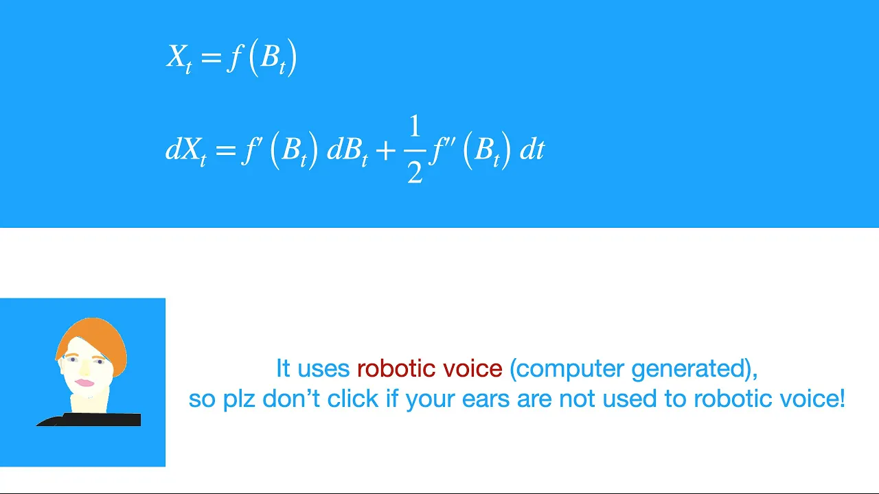
Why this video: This video offers a structured proof of Itô's Lemma. It explicitly details the Taylor series expansion of a function $f(t, X_t)$ and mathematically defends why terms containing $(dX_t)^2$ yield $dt$ while higher-order terms like $dt \cdot dW_t$ and $(dt)^2$ vanish in the limit.

---

Why this video: This rigorous derivation systematically applies Taylor's Theorem to general stochastic differentials of the form $dX_t = \mu_t dt + \sigma_t dW_t$. It is an exceptional resource for students wanting to see the formal algebra behind the multidimensional stochastic chain rule.

Knowledge Checkpoint

• Write down the single-variable and multi-variable versions of Itô's Lemma.
• Explain why the second-order derivative term ($\frac{1}{2}\frac{\partial^2 g}{\partial x^2}$) does not disappear in stochastic calculus as it does in deterministic calculus.
• Apply Itô's Lemma to compute the stochastic differential $df(W_t)$ for $f(x) = x^2$ and $f(x) = e^x$.

---

Module 5: Stochastic Differential Equations & GBM

Just as ordinary differential equations (ODEs) govern deterministic systems, Stochastic Differential Equations (SDEs) model systems evolving under continuous random shocks. This module covers how to formulate, solve, and simulate SDEs, with a heavy emphasis on Geometric Brownian Motion (GBM)—the classic mathematical model used to describe stock price dynamics.

Recommended Videos

Why this video: A clear, concise introduction to the mechanics of GBM. It explains why simple linear drift models are unrealistic for asset prices (due to the possibility of negative prices) and motivates the percentage-return SDE formulation: $dS_t = \mu S_t dt + \sigma S_t dW_t$.

---

Why this video: This lecture from the University of Chicago explains the general theory of integrating both sides of an SDE. It provides a detailed walkthrough of applying Itô's Lemma to find analytical solutions to SDEs, using the log-transformation ($Y_t = \ln S_t$) to solve the GBM SDE.

---

Why this video: Transitioning theory to practice, this tutorial walks you through simulating sample paths of Geometric Brownian Motion in Python. It demonstrates the Euler-Maruyama discretization method using numpy and matplotlib.

Knowledge Checkpoint

• Write down the standard SDE for Geometric Brownian Motion, defining the drift parameter $\mu$ and volatility parameter $\sigma$.
• Use the change of variables $F(S_t) = \ln(S_t)$ and Itô's Lemma to prove that the analytical solution to GBM is $S_t = S_0 \exp\left( (\mu - \frac{1}{2}\sigma^2)t + \sigma W_t \right)$.
• Explain why asset prices modeled by GBM are log-normally distributed and strictly positive.
• Construct a basic Euler-Maruyama simulation step for an arbitrary SDE: $X_{t+\Delta t} = X_t + \mu(X_t, t)\Delta t + \sigma(X_t, t)\Delta W$.

---

Module 6: The Black-Scholes Model

This capstone module unites everything you have learned. By modeling stock prices using Geometric Brownian Motion, applying Itô's Lemma to an option contract, and constructing a risk-free replicated portfolio (Delta Hedging), you will derive the historic Black-Scholes-Merton Partial Differential Equation (PDE) and review the resulting analytical formulas for pricing European call and put options.

Recommended Videos

Why this video: This acclaimed documentary provides the high-level historical and physical intuition behind the Black-Scholes-Merton equation. It beautifully visualizes option payoffs, dynamic hedging, and links Brownian motion in asset markets to the heat diffusion equation in physics.

---

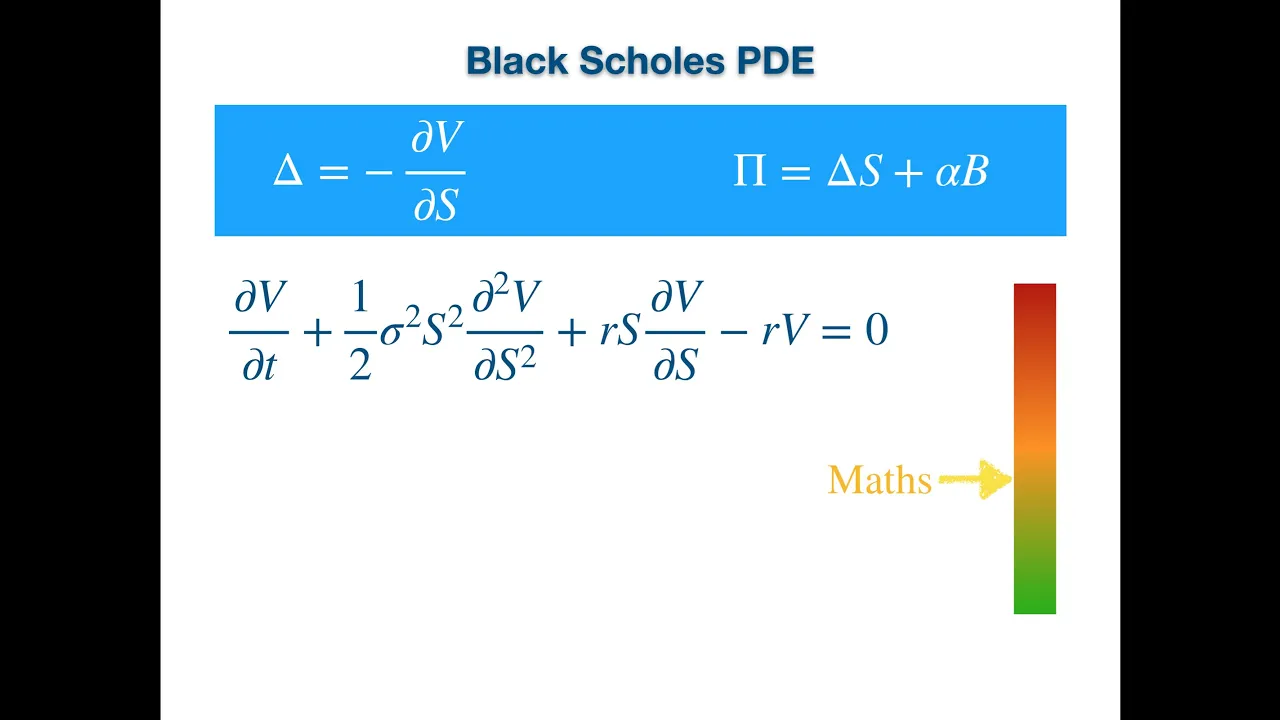
Why this video: This video contains the core mathematical derivation of the Black-Scholes PDE. It details the construction of a self-financing portfolio consisting of a long option position and a short stock position ($\Delta$-hedged), proving how the stochastic $dW_t$ term mathematically cancels out to force the portfolio to grow at the risk-free rate $r$.

---

Why this video: An academic, rigorous step-by-step breakdown from MIT OCW. This lecture mathematically defines the boundary conditions for the option at maturity ($T$) and explores the transformation of the Black-Scholes PDE into the classical heat equation to solve it analytically.

---

Why this video: To finalize your learning, this short tutorial shows how to write clean Python functions implementing the analytic solution of the Black-Scholes formula. It focuses on programmatically calculating the $d_1$, $d_2$ terms, and the cumulative normal distribution function ($N(d)$) to output option prices.

Knowledge Checkpoint

• Describe the portfolio replication argument (Delta Hedging) and why it eliminates the stochastic $dW_t$ term.
• Write down the Black-Scholes-Merton Partial Differential Equation (PDE): $\frac{\partial V}{\partial t} + rS\frac{\partial V}{\partial S} + \frac{1}{2}\sigma^2 S^2 \frac{\partial^2 V}{\partial S^2} - rV = 0$
• Define the terminal/boundary conditions for both a European call option and a European put option.
• Write down the analytical formulas for $d_1$ and $d_2$ used in the Black-Scholes pricing formulas.

---

Course Map

Below is the conceptual map and recommended learning sequence for mastering Stochastic Calculus:

---

Key People Index

• Robert Brown (1773–1858): Scottish botanist who first observed the erratic, jittery motion of pollen grains suspended in water in 1827, which was later named "Brownian motion."
• Albert Einstein (1879–1955): Formulated the first mathematical explanation of Brownian motion in 1905, showing that the random motion of particles is caused by continuous molecular bombardment, proving the existence of atoms.
• Kiyosi Itô (1915–2008): Japanese mathematician who pioneered stochastic integration and developed Itô Calculus, introducing the concept of integrating along highly non-differentiable paths.
• Fischer Black (1938–1995), Myron Scholes (1941–present), and Robert C. Merton (1944–present): Co-developed the Black-Scholes-Merton option pricing model in 1973. Scholes and Merton received the Nobel Prize in Economics in 1997 for this work (Black had passed away in 1995 and was ineligible).

---

Final Self-Assessment

Test your mastery of the complete curriculum by verifying you can perform each of the following:

• Explain how standard Brownian motion is mathematically constructed as the continuous limit of a scaled symmetric random walk.
• Define the mathematical axioms of a Wiener Process ($W_t$).
• State why the total variation of a Brownian path is infinite, and prove that its quadratic variation over $[0, t]$ is deterministically equal to $t$.
• Explain why the Riemann-Stieltjes integral fails when integrating along Brownian motion paths.
• Set up, outline, and explain the steps to prove the Itô Isometry: $\mathbb{E}[(\int_0^T X_t dW_t)^2] = \mathbb{E}[\int_0^T X_t^2 dt]$.
• Derive the differential of $f(t, W_t) = e^{W_t - \frac{1}{2}t}$ using Itô's Lemma.
• State the Stochastic Differential Equation (SDE) for Geometric Brownian Motion (GBM) and explain the economic rationale behind its percentage-drift setup.
• Solve the GBM SDE analytically using the log-transformation $Y_t = \ln S_t$.
• Outline the portfolio replication argument (Delta Hedging) used to eliminate randomness when deriving the Black-Scholes PDE.
• Write down the Black-Scholes PDE along with the terminal boundary condition for a European call option.
• Programmatically write a Python function that outputs the Black-Scholes price of a European option given $S, K, T, r,$ and $\sigma$.